University of Missouri-Columbia

Department of Electrical and Computer Engineering

ECE 7330 Introduction to Mechatronics and Robotic Vision

Fall, 2010

PROJECT #2

GENERIC ROBOT SIMULATOR

Luis Alberto Rivera Estrada

ID # 14103824

December 17^th, 2010

Abstract

The objective of this project is to develop a generic robot simulator. Several simulators of specific robots have been implemented. The program developed creates robots according to the well known D-H representations. It has several predefined robots available for the user to try. New robots are easily created by inputting the correspondent D-H parameters. To evaluate the performance of the proposed simulator, a comparison is made against Peter Corke’s Matlab Robotic Simulator.

Introduction

Having a simulator can be very helpful when designing a system. In the particular case of a robot, a simulation can help, for instance, in determining a suitable workspace for it.

There are some robot simulators available. [1] is a nice Matlab Toolbox that allows forward and inverse kinematics analysis, among others. It also allows simulating some robots. For instance, the Puma 560. [2] is another simulator that offers a nice user interface and a more detailed “CAD like” visualization of the robot. But it is restricted to one robot, the Puma 762 from the WWU Robotics Lab.

A simulator for a particular robot may include more details, like actual link dimensions and shapes, physical limitations of the robot or the workspace, special functions or tasks that the robot is programmed to do, etc. A generic robot simulator, on the other hand, is probably limited in terms of specific details, but it allows simulating important aspects like joint movements, position and orientation of end effectors, etc. of a virtually unlimited number of different robots.

The proposed simulator is based on the standard D-H representation. It allows the user to create his/her own robot by inputting the D-H parameters. The different features and limitations of the simulator will be explained throughout the report, which includes sections on technical background, description of the simulator and methods, results, conclusions and future work.

Problem Statement and Technical Background

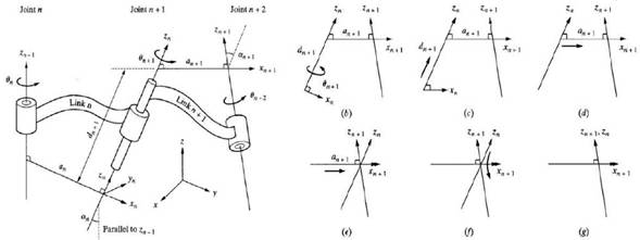
The Denavit-Hartenberg (D-H) model of representation is a simple way of modeling robot links and joints. It is assumed that a robot is made of a sequence of joints and links. The joints can be either prismatic (linear) or revolute (rotational). They can be in any order and in any plane. The links may be of any length (including zero), may be twisted or bent, and may be in any plane. So, any general set of joints and links may create a robot. [3]

To model the robot a reference frame is assigned to each joint. Matrices are defined to transform from one joint to the next. A total transformation matrix is obtained combining all the transformations from the base of the robot to the last joint (and/or possibly the end effector). [3]

[3]

The necessary motions to transform from one reference frame to the next are the following:

1. Rotation of an angle about the axis, which will make and parallel to each other.

2. Translation of a distance along the axis to make and collinear.

3. Translation of a distance along the axis to bring the origins and together.

4. Rotation of the axis an angle about the axis to align with axis to finally make frames and be exactly the same. [3]

The matrix representing the four movements is obtained by postmultiplying the four matrices representing the four movements, as follows:

Where and .

The total transformation between the base (frame 0) and the last frame (frame n, usually the hand or end effector) is .

A table of joint and link parameters (D-H table) summarizes the characteristics of a robot. The values are determined from a schematic drawing of the robot after assigning proper frames for each of the joints that constitute the robot. In essence, such a D-H table describes a robot. This is the main idea behind the generic simulator developed for this project assignment. All it takes to create and simulate a robot is to have a D-H table. In the next section I describe the actual simulator.

Description of the Simulator

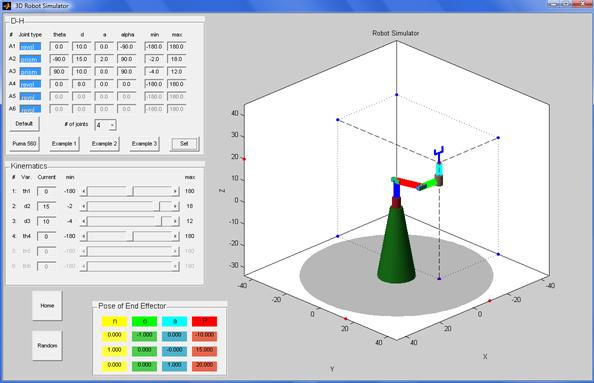
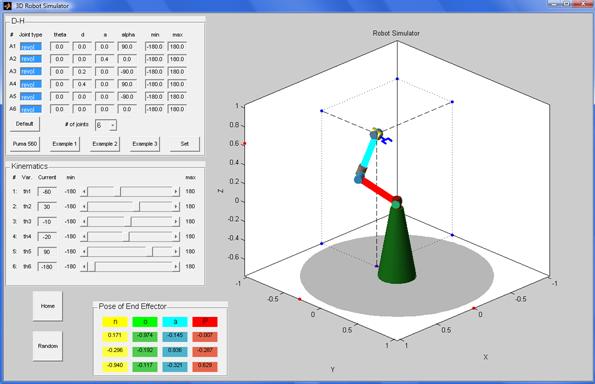
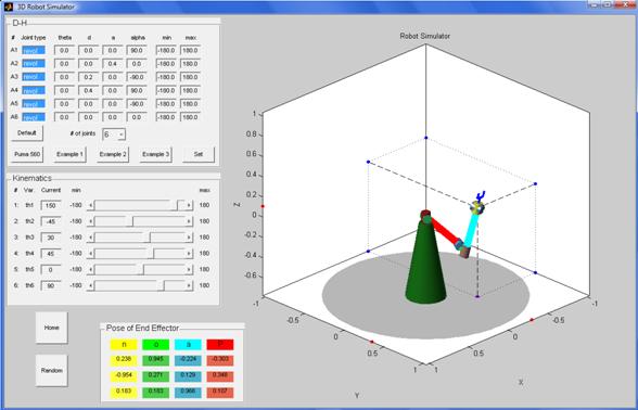
The Puma3D simulator [2] was used as a base for creating the simulator for this project. The graphical interface is illustrated next:

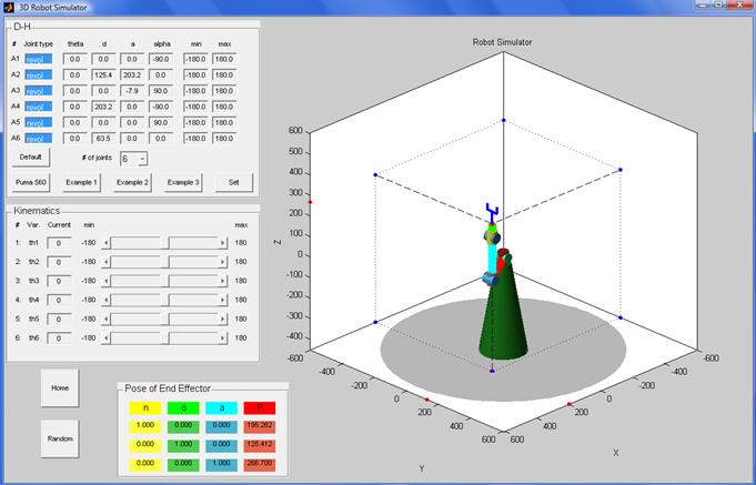
It has the following features:

· D-H table for defining the robot.

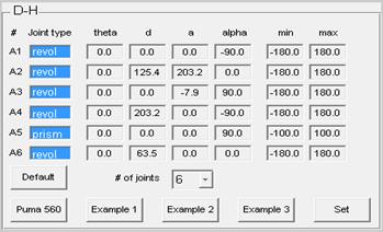
Robots with up to six joints (degrees of freedom) can be defined. The joints can be revolute or prismatic. Additional to the four parameters for each joint (q, d, a, a) it is possible to set the minimum and maximum value for the correspondent variable (q for revolute joints and d for prismatic joints). After the parameters are input, by clicking on the Set button the robot is created. The position determined by the D-H parameters (in particular, determined by the values of variables) becomes the “Home” position of the robot.

There are various pre-defined robots for the user to try. Clicking on the “Default”, “Puma 560”, “Example 1”, “Example 2” and “Example 3” will put D-H parameters in the correspondent boxes. Clicking on the set button will create the correspondent robot.

· Building the Robot.

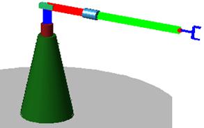
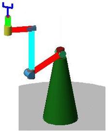
The robot consists of joints and links. Generic shapes are used for the joints. Cylinders are used for the revolute joints and prisms are used for the prismatic joints. Since there is no detailed description of the links (shape, width, etc.), thick line segments are used. Those lines connect consecutive frame origins. A simple end effector is placed at the last frame of the robot. The first origin (frame 0, corresponding to the base) is placed at the world’s origin. For visualization purposes, a (green) conical base completes the structure of the robot.

· Robot’s Workspace

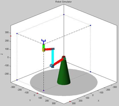
The scales of the axes adjust to the dimensions of the robot to have a good visualization of the robot. The last origin (shown in red) is projected to the ground and to the background walls. This helps in the visual localization of the end effector.

· Moving the Robot: Kinematics control.

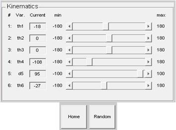
The individual joints can be manipulated in order to move the robot. A slider bar and an edit box allow changing the corresponding variables. The maximum and minimum values specified in the D-H table are reflected in the kinematics control panel. The “Random” button will produce a random movement of the robot, and the “Home” button will bring the robot to the home position.

· Position and Orientation of the End Effector

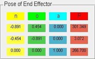
The Homogeneous transformation matrix representing the pose of the last coordinate frame is displayed in the table shown above (with the exception of the last row). Vectors n, o and a are the direction vectors of the frame, and vector P is the position vector of the frame’s origin.

Results

Next I show some of the example robots predefined. Moreover, I show a comparison between my proposed simulator and the simulator proposed in [1] for the Puma 560 robot.

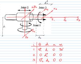
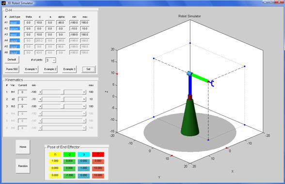
Example 1: 3 – joint robot (revolute, prismatic, revolute).

[4]

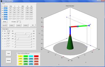
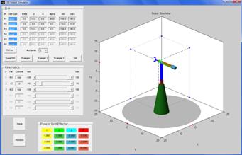
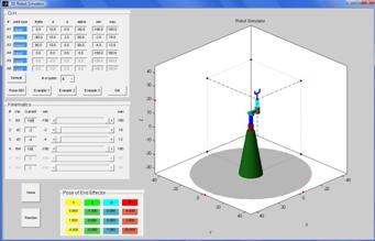
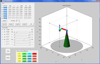
Example 2: 4 – joint robot (revolute, prismatic, prismatic, revolute).

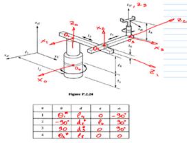[4]

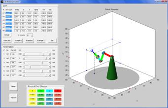
Example 3: 6 – joint robot (all revolute joints).

[4]

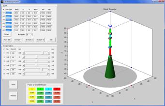
Puma 560: comparison between simulators.

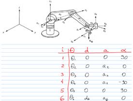
The D-H table for the Puma 560 robot according to the toolbox proposed in [1] is the following (all joints are revolute):

Shown above is the home position. Note the x, y and z coordinates of the last frame and its a direction vector. The home position according to my simulator is next:

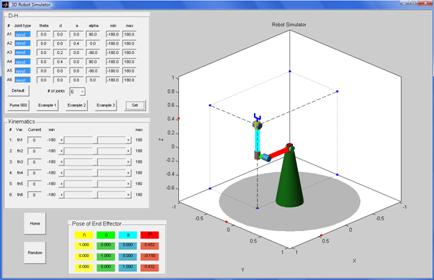
Note that both the position vector and the direction vector coincide with the correspondent vectors in Corke’s simulator. Now, consider some other configuration of the joint variables.

Comparison configuration 1:

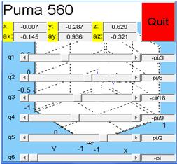
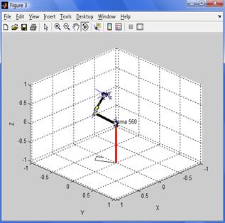
Note how the positions and orientations coincide.

Comparison configuration 2:

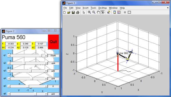
Note again how both simulators give the same position and orientation.

Conclusions and Future Work

The proposed simulator allows creating and simulating a large variety of robots, with up to six degrees of freedom. Its user friendly interface and simple D-H parameters and control panels make it easy to define and build robots, and then to move them. It offers several features that enhance the visualization of the robot and the position of the end effector. This simulator may be a useful tool for designing real robots or for academic purposes.

Future versions of the simulator may include some of the following features:

· Allow the user to save D-H parameters and to load previously saved ones.

· Allow interacting with the workspace (e.g. zooming, rotating, manipulating the axes, etc.).

· Option to place the base of the robot in different locations with respect to the world.

· Include more details of the joints and links.

· Constrain the joint variables to take physical limitations into account.

· Others.

References

1. P.I Corke “A Robotics Toolbox for MATLAB”. IEEE Robotics and Automation Magazine. No. 1, Vol. 3, March, 1996. Pp. 24 – 36.

2. PUMA3D Simulator of the Puma robot located in the Robotics Lab of Walla Walla University.

3. S. B. Niku. “Introduction to Robotics: Analysis, Systems, Applications”. Prentice Hall. United States of America, 2001.

4. G. DeSouza. Lecture notes from the course “Introduction to Mechatronics and Robotic Vision”. University of Missouri – Columbia. Fall, 2010.